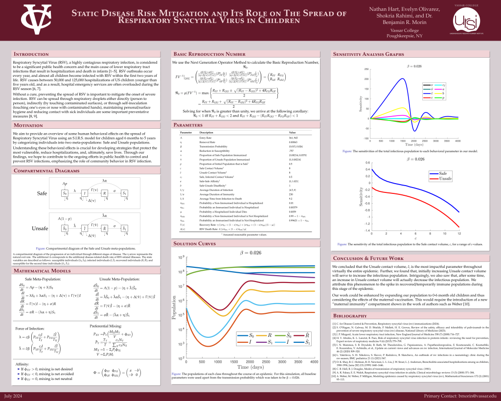
In the summer of 2024, I participated in Vassar’s Undergraduate Research Summer Institute (URSI) working with Professor Benjamin Morin and peers. Together we created a model for the spread of RSV in children ages 6mo-5yr. We are interested in human behavioral effects on the spread of the disease.
We start by considering a traditional SIRS model where susceptible individuals become infected, then can recover, and eventually become susceptible again. The unique part about our model is that we divide the population into two meta-populations: one where the children’s guardians practice safe behavior and one where guardians practice unsafe behavior. Safe behavior includes keeping children home from daycare when they are sick (something not available to every guardian), having them wear PPE, etc..
Within each meta-population different parameters represent the rates at which individuals get infected, recover, and so on. The neat part of our model was that the rate of infection in each meta-population depended on the desire of each population to interact with the other.
By running numerical simulations and sensitivity analysis we were able to predict which parameters in our model are most impactful on spreading the disease. Our results as well as the full system of differential equations describing our model are given in the poster below. We found that the contact rate of children in the unsafe meta-population was the most impactful parameter for causing infections. Next most impactful were the degrees to which the different meta-populations desired to mix with their own and avoid the others.
Differential Equations
Force of Infection
Preferential Mixing
Affinity Matrix